Simple Gearbox Generation
Taking from where we left off from the last tutorial (if you have not seen it yet, you can see it here) , in this one we are going to build a Generator for our model. The objective here is, by using network graphs, to have an understanding of the gearbox configurations regarding the position of elements, meeting all requirements imposed. All this is done using some supervised and unsupervised Machine Learning algorithms such as Decision tree and Clustering, to help us find the solutions we want. To achieve that we will build two other classes of Dessia Objects, the first is called GearBoxGenerator, where all configurations are generated, and the second one is called Clustering, which is responsible for the post treatment part of all solutions generated in the previous class.
Class GearBoxGenerator
As mentioned, this class will be used to generate all different types of configurations, and to do so we initialize it with a GearBox object, the number of inputs we want in our gearbox, the maximum number of shaft assemblies we are willing to have in it, as well as the maximum number of gears. To make all the coding process simpler and more understandable, we have divided it in smaller parts, building a method for each one, which are described below.
class GearBoxGenerator(DessiaObject):
     _standalone_in_db = True

     def __init__(self, gearbox: GearBox, number_inputs:int,
                  max_number_shaft_assemblies: int,
                  max_number_gears: int, name:str = ''):
        self.gearbox = gearbox
        self.number_inputs = number_inputs
        self.max_number_shaft_assemblies = max_number_shaft_assemblies
        self.max_number_gears = max_number_gears
        DessiaObject.__init__(self,name=name)
Method generate connections
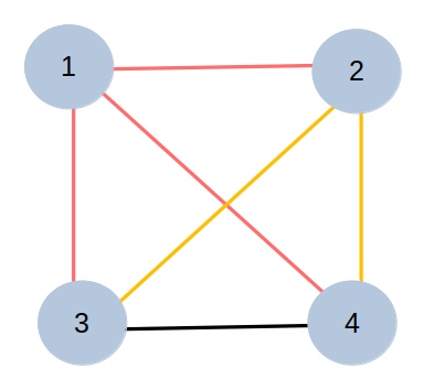
The objective of this method is to build, with the help of a decision tree, all possible gearbox configurations where two main parameters are used: the number of shaft assemblies and number of gears. The Decision Tree is used to define where each gear should be placed in the gearbox, i.e. which shafts each gear connects. In order to do this, these possible connections were created first, knowing that all shafts should be connected to each other without repeated combinations, for example: for the case where we have a maximum number of shaft assemblies of 4, a gear can be placed in any of the following connections: (1,2), (1,3), (1,4), (2,3),(2,4),(3,4), where (1,2) means in fact the connection between the shaft one and shaft two. It is also very well represented in the image below.
Also, we want it to be as dynamic and generate as much viable solutions as possible, meaning that we want the total number of elements to vary between a minimum and a maximum number. To do that, we add a new connection to our list, representing an empty option. This list of possible connections is then used to build the list of nodes for the decision tree, which is its length, where each element represents a stage of the decision tree, which for instance is a gear, and the value for that element represents how many possible outcomes it can bear. And finally the decision tree is built using the RegularDecisonTree algorithm from DessIA's dectree module.
def generate_connections(self):
        list_node = []
        connections = []
        list_dict_connections = []

        for i in range(self.max_number_shaft_assemblies):
            for j in range(self.max_number_shaft_assemblies):
                if i < j:
                    connections.append((i+1, j+1))
        connections.append(None)
        for gear in range(self.max_number_gears):
            list_node.append(len(connections))
        tree = dt.RegularDecisionTree(list_node)
        while not tree.finished:
              valid = True
              node = tree.current_node
              new_node = []
              for nd in node:
                  if nd != len(connections)-1:
                      new_node.append(nd)
              if len(new_node) == 0 :
                  valid = False
              if len(node) == self.max_number_gears and valid:
                  dict_connections = {}
                  for i_node, nd in enumerate(new_node):
                      dict_connections['G' + str(i_node+1)] = connections[nd]
                  list_dict_connections.append(dict_connections)
              tree.NextNode(valid)
        return list_dict_connections
During the decision tree construction, because there is no element differentiation between the input and output, many equivalent solutions were noticed, where nodes would just interchange positions. For example, using the same parameters as presented previously, we could have one gearbox configuration being {gear 1: (1,2), gear 2: (1,2), gear 3: (2,3), gear 4: (3,4)} and another one {gear 1: (1,3), gear 2: (1,3), gear 3: (2,3), gear 4: (2,4)} which are especially the same if we consider shaft 2 equivalent to shaft 3. To work around that problem, a condition was implemented in the while loop for the decision three to eliminate this kind of duplicate solutions. It works in such a way to avoid coming back to an inferior index, eliminating the second configuration mentioned for example, where from shaft 3 in gear2 it comes back to shaft 2 in gear 3. Finally, if the solution is valid, a dictionary is built with the corresponding gear and where it is placed. You can visualize this modification in the code box below.
def generate_connections(self):
        list_node = []
        connections = []
        list_dict_connections = []

        for i in range(self.max_number_shaft_assemblies):
            for j in range(self.max_number_shaft_assemblies):
                if i < j:
                    connections.append((i+1, j+1))
        connections.append(None)
        for gear in range(self.max_number_gears):
            list_node.append(len(connections))
        tree = dt.RegularDecisionTree(list_node)
        while not tree.finished:
              valid = True
              node = tree.current_node
              new_node = []
              for nd in node:
                  if nd != len(connections)-1:
                      new_node.append(nd)
              if len(new_node) >  1:
                  if connections[new_node[-1]][0] != connections[new_node[-2]][0]:
                      if connections[new_node[-1]][0] != connections[new_node[-2]][1]:
                          valid = False
              if len(new_node) == 0 :
                  valid = False
              if len(node) == self.max_number_gears and valid:
                  dict_connections = {}
                  for i_node, nd in enumerate(new_node):
                      dict_connections['G' + str(i_node+1)] = connections[nd]
                  list_dict_connections.append(dict_connections)
              tree.NextNode(valid)
        return list_dict_connections
Method Generate Paths
Once all possible architectures are generated, the next step is to sort them by number of speeds, meaning: which ones of those solutions have the exact number of ratios we are looking for in our gearbox. To do so, we use the python Networkx package which is very helpful when we want to use node graph representation for our problems, since it already has built-in functions to do certain tasks, such as searching how many different paths there are in a graph when going from a point to another. To accomplish this, we go through each one of the configurations obtained with the decision tree and firstly we build a non directed networkx graph, placing a gear between each two shafts. Also, for posterior identification purposes while searching for duplicate solutions, a node type was assigned to each node, 'Input Shaft' and 'Output Shaft' for the input and output shaft respectively, as well as just 'Shaft' for any shaft between the input and output, and also 'Gear' for all gears.
def generate_paths(self, list_gearbox_connections):
        list_gearbox_connections = self.generate_connections()
        list_gearbox_graphs = []
        list_paths = []
        list_paths_edges = []
        list_dict_connections = []
        for gearbox_connections in list_gearbox_connections:
            gearbox_graph = nx.Graph()
            for gearbox_connection in gearbox_connections:
                gearbox_graph.add_edge('S'+str(gearbox_connections[gearbox_connection][0]), gearbox_connection)
                gearbox_graph.add_edge(gearbox_connection,'S'+str(gearbox_connections[gearbox_connection][1]))

            number_shafts = 0
            number_gears = 0
            input_shaft = 'S'+str(min([shaft for gearbox_connection in \\
                                       gearbox_connections.values() for shaft in gearbox_connection]))
            output_shaft = 'S' + str(max([shaft for gearbox_connection in \\
                                          gearbox_connections.values() for shaft in gearbox_connection]))
            for node in gearbox_graph.nodes():
                if node == input_shaft:
                    gearbox_graph.nodes()[node]['Node Type'] = 'Input Shaft'
                    number_shafts += 1
                elif node == output_shaft:
                    gearbox_graph.nodes()[node]['Node Type'] = 'Output Shaft'
                    number_shafts += 1
                elif 'S' in node:
                    gearbox_graph.nodes()[node]['Node Type'] = 'Shaft'
                    number_shafts += 1
                else:
                    gearbox_graph.nodes()[node]['Node Type'] = 'Gear'
                    number_gears += 1
The second part of the method is dedicated to validating the solutions. With all the information passed to the graph, it is possible to calculate all simple paths between the input and output, and if it corresponds to the number of ratios desired, then the first requirement has already been satisfied. Next it is verified that every node in the graph is present in at least one of these paths, otherwise it means there are nodes, i.e. a shaft or a gear, which are not being used in the system, and we do not want this to happen so that solution is set to not valid. The final step is to verify that we will not have any duplicate solution, which is the hardest part if you want to create your own algorithm to sort all kinds of solutions, because very often there may be a large number of them and the best way to take them all into account is not always obvious. Therefore, to solve that, because we had assigned a node type for each node of the graph, it is then possible to use a networkx isomorphism algorithm relating to the node type 'Shaft', for the current graph and all previous valid ones. Finally, if all these conditions are valid, the solution is saved in a list for the next phase. Alongside that, some graph parameters are also saved for post treatment purposes, by way of example the total number of shafts, the standard deviation for the input/gears distance and density of the graph.
            paths = []
            count = 0
            average_lengths = []
            for path in nx.all_simple_paths(gearbox_graph, input_shaft, output_shaft):
                paths.append(path)
                average_lengths.append(len(path))
                count += 1
            paths_edges = []
            for path in map(nx.utils.pairwise, paths):
                paths_edges.append(list(path))

            if count == len(self.gearbox.speed_ranges):
                valid = True
                gears_path_lengths = []
                for node in gearbox_graph.nodes():
                    if node not in [path_node for path in paths for path_node in path]:
                        valid = False
                    if gearbox_graph.nodes()[node]['Node Type'] == 'Gear':
                        gears_path_lengths.append(nx.shortest_path_length(gearbox_graph, input_shaft,node))
                for graph in list_gearbox_graphs:
                    node_match = iso.categorical_node_match('Node Type', 'Shaft')
                    if nx.is_isomorphic(gearbox_graph, graph, node_match= node_match):
                        valid = False
                if valid:
                    gearbox_graph.graph['Average length path'] = mean(average_lengths)
                    gearbox_graph.graph['Number of shafts'] = number_shafts
                    gearbox_graph.graph['Number of gears'] = number_gears
                    gearbox_graph.graph['Standard deviation distante input/gears'] = np.std(gears_path_lengths)
                    gearbox_graph.graph['Density'] = nx.density(gearbox_graph)
                    list_gearbox_graphs.append(gearbox_graph)
                    list_paths.append(paths)
                    list_paths_edges.append(paths_edges)
                    list_dict_connections.append(gearbox_connections)

        return list_gearbox_graphs
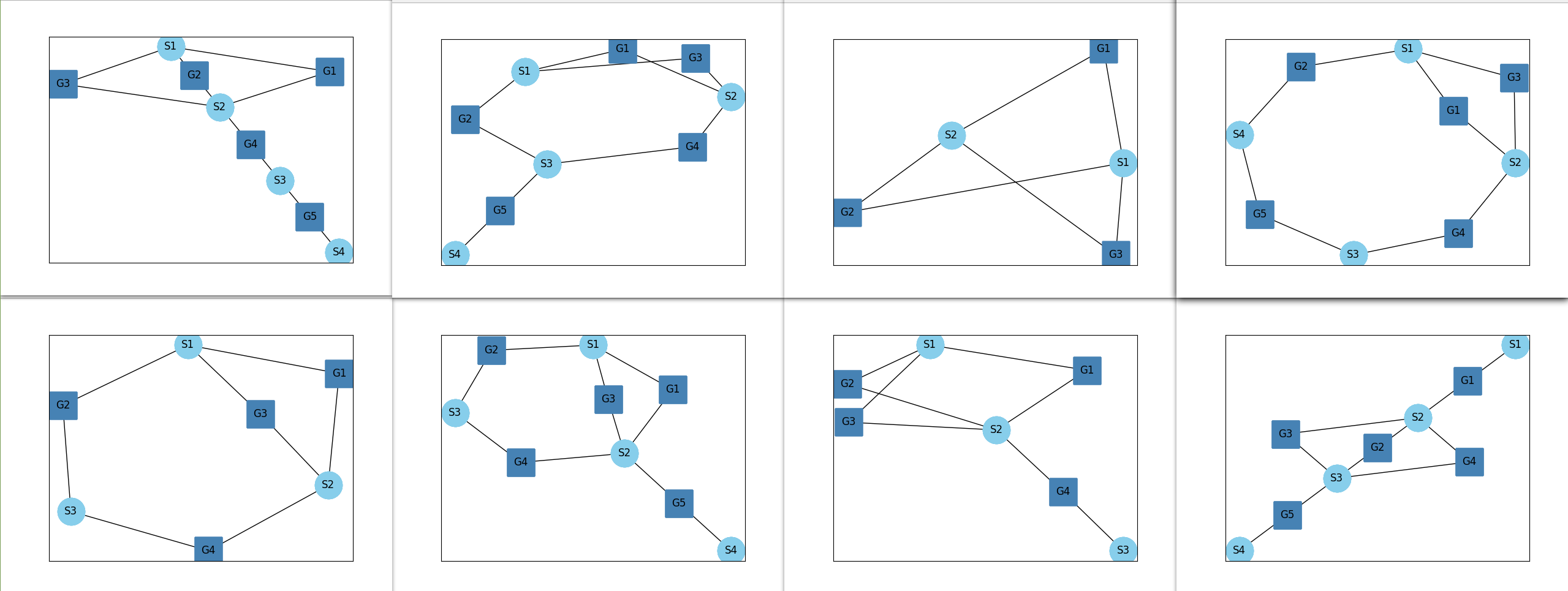
Some of the valid architectures generated by this method are shown below:
Method Clutch Analysis
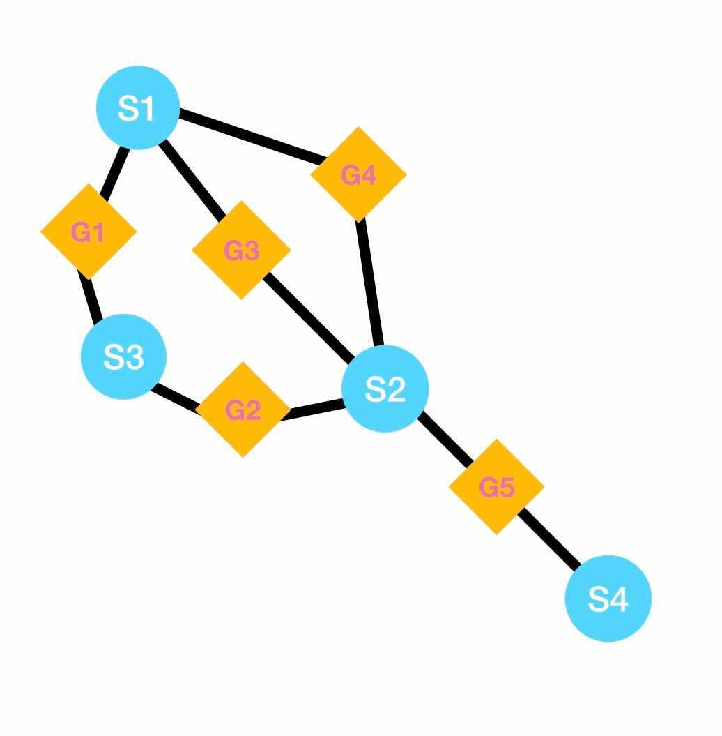
As it was possible to notice with the results given by the previous method, most of them have cycles, which means that a shaft may be shared by multiple gears. In cases like this, we must find a way to make sure that when a ratio is activated, the others are not, i.e., no movement goes through more than one path at a time. To do so, it was decided to add some clutches to our model, and the objective of this method is to exactly decide where it should be placed in the cycle. To explain the reasoning of this method, consider the cycles [S1, G1, S3, G2, S2, G4] and [S1, G3, S2, G4] for the configuration of the image shown below. There should be a clutch for each cycle, furthermore, each can be placed one after the other in any shaft present in the cycle, resulting in a few different combinations for the clutches positions, for this particular example we have [(S1, S1), (S1, S2), (S3, S1), (S3, S2), (S2, S1), (S2, S2)] as possible positions for the two clutches.
To find these combinations, it is first needed to find these cycles in the graphs, which is done with the help of the 'cycle_basis()' Networkx function and then the 'product()' function from itertools is used. Once this part is done, we go through each combination found and a node attribute is set to 'True' for the corresponding shaft nodes, and in addition to that a dictionary is built to keep track of the gear nodes coming before and after the shaft node having a clutch, this is important because after it will be useful to determine between which two gears a clutch should be introduced. Finally some other parameters like the average and standard deviation for input/clutch distance. You can see the corresponding method in the box below.
def clutch_analisys(self, list_path_generated_graphs):
        new_list_gearbox_graphs = []
        list_clutch_combinations = []
        list_cycles = []
        list_dict_clutch_connections = []
        for graph in list_path_generated_graphs:
            for node in graph.nodes():
                if graph.nodes()[node]:
                    if graph.nodes()[node]['Node Type'] == 'Input Shaft':
                        input_shaft = node
            cycles = nx.cycle_basis(graph, root = input_shaft)
            list_cycles.append(cycles)
            list_cycle_shafts = []
            for cycle in cycles:
                cycle_shafts = []
                for node in cycle:
                    if 'S' in node:
                        cycle_shafts.append(node)
                list_cycle_shafts.append(cycle_shafts)
            clutch_combinations = list(product(*list_cycle_shafts))
            list_clutch_combinations.append(clutch_combinations)
            for clutch_combination in clutch_combinations:
                graph_copy = copy.deepcopy(graph)
                dict_clutch_connections = {}
                for i_cycle, cycle in enumerate(cycles):
                    for i_node, node in enumerate(cycle):
                        if clutch_combination[i_cycle] == node:
                            if clutch_combination[i_cycle] == cycle[-1]:
                                dict_clutch_connections[i_cycle + 1] = (cycle[0], cycle[i_node-1])
                                graph_copy.nodes()[node]['Clutch'] = True
                            else:
                                dict_clutch_connections[i_cycle + 1] = (cycle[i_node+1], cycle[i_node-1])
                                graph_copy.nodes()[node]['Clutch'] = True
                clutch_path_lengths = []
                for node in graph_copy.nodes():
                    if 'Clutch' in list(graph_copy.nodes()[node].keys()):
                        clutch_path_lengths.append(nx.shortest_path_length(graph_copy, input_shaft, node))
                graph_copy.graph['Average distance clutch-input'] = mean(clutch_path_lengths)
                graph_copy.graph['Standard deviation distante input/cluches'] = np.std(clutch_path_lengths)
                list_dict_clutch_connections.append(dict_clutch_connections)
                new_list_gearbox_graphs.append(graph_copy)
        return new_list_gearbox_graphs, list_dict_clutch_connections, list_clutch_combinations, list_cycles
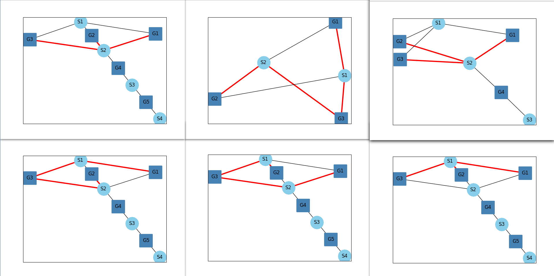
The results of this method is shown below. In these examples, two red edges connected to a shaft node means there is clutch there.
Method Generate
Finally, we get to the last method for our final solutions. The objective of this method is to take everything we have developed so far, eliminate some invalid solutions and also provide a more detailed representation for the valid ones. To achieve that, we go through every graph given by the last clutch_analisys method and a first validation is done using the dictionary containing the nodes coming before and after a shaft-with-clutch node, where it is checked if two connections are the same. This verification is done because there may exist solutions in which two or more clutches are positioned at the exact same place, which is obviously an outcome we do not want to have.
     def generate(self):
        generate_connections = self.generate_connections()
        generate_paths = self.generate_paths(generate_connections)
        clutch_analisys = self.clutch_analisys(generate_paths)
        list_gearbox_solutions = []
        clutch_gearbox_graphs = clutch_analisys[0]
        list_clutch_connections = clutch_analisys[1]
        list_clutch_combinations = [clutch_combination for clutch_combinations in clutch_analisys[2] for clutch_combination in clutch_combinations]
        list_clutch_gearbox_graphs = []
        for i_graph, graph in enumerate(clutch_gearbox_graphs):
            valid = True
            graph_copy = copy.deepcopy(graph)
            clutch_connections = list_clutch_connections[i_graph]
            for i, connections in enumerate(list(list_clutch_connections[i_graph])):
                if i!=0:
                    if list_clutch_connections[i_graph][i+1] ==  list_clutch_connections[i_graph][i]:
                        print(list_clutch_connections[i_graph][i+1],list_clutch_connections[i_graph][i])
                        valid = False
                        break
            if not valid:
                continue
            .
            .
            .
The next step is to go in every node in the graph containing a clutch and do some modifications to the graph around that node always using the connection information in the dictionary mentioned. The main objective here is to eliminate the edges between the shaft nodes and the connected gear nodes, and then add another intermediate node between the gear and shaft nodes, representing a secondary shaft, as shown for the two graphs below. These secondary shafts are later connected to one another to represent a clutch between two gears connected to that shaft node. Just before saving the solutions, one last verification is done for the configurations which do not have any intermediate shaft node for all paths from the input shaft to the output shaft so to avoid any possible cases where there is always an active path.
            .
            .
            .
            for node in graph.nodes():
                if 'Clutch' in list(graph.nodes()[node].keys()):
                    for edge in graph.edges():
                        if node in edge:
                            clutch_link_values = [value for values in clutch_connections.values() for value in values]
                            if edge[0] in clutch_link_values or edge[1] in clutch_link_values:
                                graph_copy.remove_edge(edge[0], edge[1])
                                if 'S' in edge[0]:
                                    graph_copy.add_edge(edge[1],edge[0]+'-'+edge[1])
                                    graph_copy.add_edge(edge[0], edge[0]+'-'+edge[1])
                                else:
                                    graph_copy.add_edge(edge[0],edge[1]+'-'+edge[0])
                                    graph_copy.add_edge(edge[1], edge[1]+'-'+edge[0])
            for node in graph_copy.nodes():
                if graph_copy.nodes()[node]:
                    if graph_copy.nodes()[node]['Node Type'] == 'Input Shaft':
                        input_shaft = node
                    if graph_copy.nodes()[node]['Node Type'] == 'Output Shaft':
                        output_shaft = node
            paths = nx.all_simple_paths(graph_copy, input_shaft, output_shaft)

            for path in paths:
                if not any(('S' in node and 'G' in node) for node in path):
                    valid = False
                    print('problem: ', list_clutch_combinations[i_graph])

            for i_shaft, shaft in enumerate(list_clutch_combinations[i_graph]):
                graph_copy.add_edges_from([(shaft+'-'+ clutch_connections[i_shaft+1][0],
                                            shaft+'-'+ clutch_connections[i_shaft+1][1],
                                            {'Clucth': True})])
            if valid:
                gearbox = self.gearbox.copy()
                gearbox.update_gb_graph(graph_copy)
                list_gearbox_solutions.append(gearbox)
                list_clutch_gearbox_graphs.append(graph_copy)

        return list_gearbox_solutions, list_clutch_gearbox_graphs
Some of the final results are shown in the figure below.
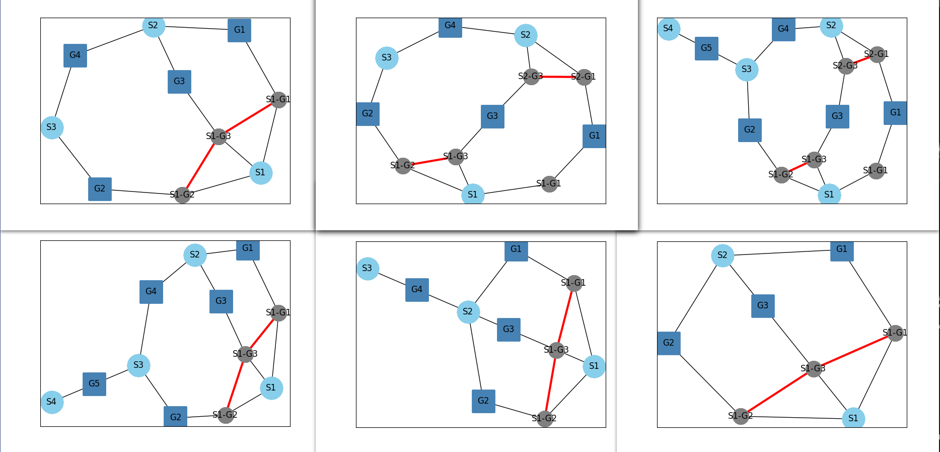
Method Draw Graph
The draw graph method is a particular one responsible for shaping and plotting the different results using some networkx functions. Essentially what this method does is that it gives differents shapes and colors to the different elements of our graph, for example, as you might have realized the shaft nodes are light blue circles and the gears are a little darker blue squares, as for the edges representing the clutches, they were set in red. This is possible because the networkx kamada_kawai_layout() provides all positions for all elements of the graph, which may be accessed later on to change some particular elements. A condition was also introduced in case we do not want to see all results.
    def draw_graph(self, graphs_list: List[nx.Graph], max_number_graphs:int = None):

        for i, graph in enumerate(graphs_list):
            plt.figure()
            gears = []
            shafts = []
            S_G = []
            for node in graph.nodes():
                for node in graph.nodes():
                    if 'S' in node and 'G' in node:
                        S_G.append(node)
                    elif 'S' in node and 'G' not in node:
                        shafts.append(node)
                    else:
                        gears.append(node)
            edges = []
            edges_clutch =[]
            for edge in graph.edges():
                if graph.edges()[edge]:
                    edges_clutch.append(edge)
                else:
                    edges.append(edge)

            pos = nx.kamada_kawai_layout(graph)

            nx.draw_networkx_nodes(graph, pos, shafts, node_color='skyblue', node_size=1000)
            nx.draw_networkx_nodes(graph, pos, S_G, node_color='grey', node_size=500)
            nx.draw_networkx_nodes(graph, pos, gears, node_shape = 's', node_color='steelblue', node_size=1000)
            nx.draw_networkx_edges(graph, pos, edges_clutch,edge_color='red', width= 3)
            nx.draw_networkx_edges(graph, pos, edges)
            labels = {element: element for element in  shafts + S_G + gears}
            nx.draw_networkx_labels(graph, pos, labels=labels)
            if max_number_graphs is not None:
                if i >= max_number_graphs:
                    break
Class Clustering
With all the results given by the class Generator, it was important to find a way to analyse them in a relatively simple way, so it was decided to use some clustering algorithms to assemble similar solutions in smaller groups regarding a few parameters. The class is initialized with only two main parameters, a list of gearbox objects (the result from the generate method explained above), and a name. To build the clusters some of the parameters saved during the generator procedures were used. Some of the parameters used are the average distance between input/output, the standard deviation for the input/gears distance, the average input/clutch distance, as well as the ratio input-output distance to the total number of shafts and the density of the given graph. So in order to do this, firstly, all these parameters were stored in a dictionary and then transformed into a pandas data frame so we can manipulate it more easily.
class Clustering(DessiaObject):
    standalone_in_db  = True
    def __init__(self, gearboxes:List[GearBox], name:str=""):
        self.gearboxes = gearboxes
        DessiaObject.__init__(self,name=name)
        dict_features = {}
        for gearbox in self.gearboxes:
            for attr in gearbox.graph.graph.keys():
                if attr in dict_features.keys():
                    variable = dict_features[attr]
                    variable.append(gearbox.graph.graph[attr])
                    dict_features[attr] = variable
                else:
                    dict_features[attr] = [gearbox.graph.graph[attr]]
        self.dict_features = dict_features
        self.df = pd.DataFrame.from_dict(self.dict_features)
Some methods were created to help us along the way.
Method normalize
To make sure we will not have any issue related to a parameter having a stronger influence while building the clusters in case its scale size is more important compared to others, we use the MinMaxScaler from sklearn to normalize our dataframe to values between zero and one.
    def normalize(self, df):
        scaler = MinMaxScaler()
        scaler.fit(df)
        df_scaled = scaler.fit_transform(df)
        return df_scaled
Method DBSCAN
For this study, we used the DBSCAN from sklearn, a density-based clustering non-parametric algorithm: given a set of points in some space, it groups together points that are closely packed together (points with many nearby neighbors), marking as outliers points that lie alone in low-density regions (whose nearest neighbors are too far away). While using the dbscan algorithm, we must provide some important parameters such as the epsilon value, that is the maximum distance between two samples for one to be considered as in the neighborhood of the other, which for our case was set to 0.525 because we normalized our data and it is a parameter you can change according to your needs in order to better represent our data. There is also the minimum number of samples for it to be considered a core point as well as what metric you want to use to calculate distances (euclidean, cityblock, cosine) as well as other parameters. This method returns the labels with the corresponding cluster for each element along side with the total number of clusters.
    def dbscan(self, df):

        db = DBSCAN(eps=0.525, min_samples=3,
                    # metric= 'cityblock'
                    )
        db.fit(df)
        labels =[int(label) for label in list(db.labels_)]
                # Number of clusters in labels, ignoring noise if present.
        n_clusters = len(set(labels)) - (1 if -1 in labels
                                                   else 0)
        print('Estimated number of clusters:', n_clusters)
        return labels, n_clusters
Method family groups
The objective of building clusters was also to help us during the post treatment analysis in the Dessia platform, so in order to do that we must group all gearboxes belonging to one cluster together, so their indexes may change. Therefore this method is responsible for all processes of reordering the gearbox objects and also every other parameter that must be consistent with the gearboxes indexes. It is also important to mention that because we have a multidimensional clustering for using more than two parameters, it ends up not being very easy to have a visual representation of them, so to solve that we use a multidimensional scaling algorithm (MDS) from sklearn which is used to evaluate the level of similarity of individual cases of a dataset. The way it works is essentially that given a distance matrix with the distances between each pair of objects in a set, and a chosen number of dimensions, N, the MDS algorithm places each object into a N-dimensional space (a lower-dimensional representation) such that the between-object distances are preserved as well as possible, allowing us to have ultimately a 2D representation of our clusters and these values are also reordered to match with the new gearboxes indexes. The method returns all lists of important elements reordered along side with a list of the different clusters.
    def family_groups(self, df, labels):
        encoding_mds = MDS()
        matrix_mds = [element.tolist() for element in encoding_mds.fit_transform(df)]
        clusters = []
        list_indexes_groups =[]
        gearboxes_indexes = []
        index = 0
        cluster_labels_reordered = []
        for label in labels:
            if label not in clusters:
                clusters.append(label)
        for j, cluster in enumerate(clusters):
            indexes = []
            for i, label in enumerate(labels):
                if cluster == label:
                    cluster_labels_reordered.append(label)
                    indexes.append(index)
                    index += 1
                    gearboxes_indexes.append(i)
            list_indexes_groups.append(indexes)
        new_gearboxes_order =[]
        new_matrix_mds = []
        for index in gearboxes_indexes:
            new_gearboxes_order.append(self.gearboxes[index])
            new_matrix_mds.append(matrix_mds[index])
        return clusters, cluster_labels_reordered, list_indexes_groups, new_gearboxes_order, new_matrix_mds
Method Plot Clusters
The method plot_data is responsible for displaying the clusters using our module plot_data, where a Scatter plot was used to display the clustering itself but furthermore a ParallelPlot was also used with all the parameters used to build the clusters, which may be very useful during the analysis of the clusters generated. Firstly we go through each point of the matrix generated by the multidimensional scaling algorithm and they are all stored along with the clustering parameters to build a list of points. The next step is to build the family of points corresponding to each cluster generated, assigning a different color to each cluster. Once the two types of graphs were generated, they are assembled in a MutiplePlot. If you want more details on how the module plot_data works, please check our tutorial on this topic by clicking here (opens in a new tab).
@plot_data_view(selector="MultiPlot")
def plot_data(self, reference_path: str = "#", **kwargs):
    colors = [RED, GREEN, ORANGE, BLUE, LIGHTSKYBLUE,
              ROSE, VIOLET, LIGHTRED, LIGHTGREEN,
              CYAN, BROWN, GREY, HINT_OF_MINT, GRAVEL]
    all_points = []
    for i, point in enumerate(self.matrix_mds):
        point = {
            'x': point[0], 'y': point[1],
            'Aver path': self.gearboxes_ordered[i].average_path_length,
            'Aver L clutch-input': self.gearboxes_ordered[i].average_clutch_distance,
            'ave_l_ns': self.gearboxes_ordered[i].ave_l_ns,
            'Number shafts': self.gearboxes_ordered[i].number_shafts,
            'Std input_cluches': self.gearboxes_ordered[i].std_clutch_distance,
            'Density': self.gearboxes_ordered[i].density,
            'Cluster': self.labels_reordered[i]
        }
        all_points.append(plot_data.Sample(values=point, reference_path=f"{reference_path}/#/{i}"))

    point_families = []
    for i, indexes in enumerate(self.list_indexes_groups):
        color = colors[i]
        point_family = plot_data.PointFamily(
            point_color=color, point_index=indexes,
            name='Cluster '+str(self.clusters[i])
        )
        point_families.append(point_family)

    all_attributes = ['x', 'y', 'Aver path', 'Aver L clutch-input',
                      'ave_l_ns', 'Number shafts',
                      'Std input_cluches', 'Density', 'Cluster']

    tooltip = plot_data.Tooltip(attributes=all_attributes)

    edge_style = plot_data.EdgeStyle(color_stroke=BLACK, dashline=[10, 5])

    plots = [plot_data.Scatter(tooltip=tooltip,
                               x_variable=all_attributes[0],
                               y_variable=all_attributes[1])]

    rgbs = [[192, 11, 11], [14, 192, 11], [11, 11, 192]]
    plots.append(plot_data.ParallelPlot(edge_style=edge_style,
                                        disposition='vertical',
                                        axes=all_attributes,
                                        rgbs=rgbs))
    clusters = plot_data.MultiplePlots(plots=plots,
                                       elements=all_points,
                                       point_families=point_families,
                                       initial_view_on=True)
    return clusters
Workflow
The workflow for this tutorial has not changed much compared to that of the Simple Gearbox Tutorial. In fact, the only changes made were the elimination of the blocks related to the Optimizer and to the WLTPCycle and the introduction of a block for the Generator, one for the method generate from the generator and another one for the Clustering class. Furthermore the display block was changed from a Multiplot for a Display. In the code box below only the modifications mentioned are shown.
import tutorials.tutorial10 as objects
from dessia_common.workflow.core import Workflow, Pipe, WorkflowRun
from dessia_common.workflow.blocks import InstantiateModel, ModelMethod, PlotData
from dessia_common.typings import PlotDataType, MethodType

block_generator = InstantiateModel(objects.GearBoxGenerator, name='Gearbox Generator')
block_generate = ModelMethod(MethodType(class_=objects.GearBoxGenerator, name='generate'), name='Generate')
block_efficiencymap = InstantiateModel(objects.EfficiencyMap, name='Efficiency Map')
block_engine = InstantiateModel(objects.Engine, name='Engine')
block_gearbox = InstantiateModel(objects.GearBox, name='Gearbox')
block_cluster = InstantiateModel(objects.Clustering, name='Clustering')

display = PlotData(selector=PlotDataType(class_=objects.Clustering, name="cluster plot"), name='Display')

block_workflow = [block_generator, block_generate, block_gearbox, block_engine, block_efficiencymap,
                  block_cluster,
                  display
                  ]
pipe_workflow = [Pipe(block_generator.outputs[0], block_generate.inputs[0]),
                 Pipe(block_gearbox.outputs[0], block_generator.inputs[0]),
                 Pipe(block_engine.outputs[0], block_gearbox.inputs[0]),
                 Pipe(block_efficiencymap.outputs[0], block_engine.inputs[0]),
                 Pipe(block_generate.outputs[0], block_cluster.inputs[0]),
                 Pipe(block_cluster.outputs[0], display.inputs[0])
                 ]

workflow = Workflow(block_workflow, pipe_workflow, block_generate.outputs[0])

.
.
.

input_values = {workflow.input_index(block_generator.inputs[1]): 2,
                workflow.input_index(block_generator.inputs[2]): 5,
                workflow.input_index(block_generator.inputs[3]): 5,
                workflow.input_index(block_gearbox.inputs[1]): speed_ranges,
                workflow.input_index(block_engine.inputs[1]): setpoint_speed,
                workflow.input_index(block_engine.inputs[2]): setpoint_torque,
                workflow.input_index(block_efficiencymap.inputs[0]): engine_speeds,
                workflow.input_index(block_efficiencymap.inputs[1]): engine_torques,
                workflow.input_index(block_efficiencymap.inputs[2]): mass_flow_rate_kgps,
                workflow.input_index(block_efficiencymap.inputs[3]): fuel_hv,
                }

workflow_run = workflow.run(input_values)