Piping in constraint environment
1 - Introduction
The objective of this tutorial is to generate and optimize a pipe that is in a constraint environment. Indeed, we will force the pipe to pass through 4 points and force its neutral fiber minimal radius to be superior than an imposed value.
2 - Build the bot in 4 steps
Before beginning, you have access to tutorial5 in the tutorials folder cloned as explained in the first tutorial. We will apply DessIA method to find the best solution to our problem.
2.1 - Describe your engineering system
2.1.1 - Constraint environment
First of all, we need to import some packages :
import volmdlr as vm
import volmdlr.primitives3d as p3d
import volmdlr.faces

from dessia_common.core import DessiaObject, PhysicalObject
from typing import List
In our problem, we want to generate and optimize solutions regarding a constraint environment. In this case, we want to install a pipe with a housing, a support. We define this environment with Housing method that needs a list of faces (the environment) and the spatial environment origin.
class Housing(PhysicalObject):
    _standalone_in_db = False

    def __init__(self, faces: List[vm.faces.Face3D], origin: vm.Point3D,
                 name: str = ''):
        self.origin = origin
        self.faces = faces
        PhysicalObject.__init__(self, name=name)

    def volmdlr_primitives(self):
        for face in self.faces:
            face.translation(self.origin)
        return self.faces
How to create a face ?
Faces are created thanks to volmdlr which will be called thanks to 'vm.'.
- Create a frame :
frame_center = vm.Point3D(0, 1, 0) # x,y,z position
dir1, dir2, dir3 = vm.Vector3D(1,0,0), vm.Vector3D(0,1,0), vm.Vector3D(0,0,1) # vector's direction

frame = vm.Frame3D(frame_center, dir1, dir2, dir3)
- Create a plane where the face will be :
plane = vm.surfaces.Plane3D(frame) # from vm.surfaces we create a plane thanks to frame. Plane will be based on dir1 and dir2
- Create a Surface2D :
out_contour = vm.wires.ClosedPolygon2D([vm.Point2D(-1, -1), vm.Point2D(1, -1), vm.Point2D(1, 1), vm.Point2D(-1, 1)])
surface2d = vm.surfaces.Surface2D(outer_contour=out_contour, inner_contours=[]) #Our contour doesn't have hole this is why inner_contours=[]
- Create a face :
planeface = vm.faces.PlaneFace3D(surface3d=plane, surface2d=surface2d) #We put the surface2d on the plane and we have 3D surface
- 3D display is available if your class contains a 'volmdlr_primitives' method in it. This method has to return volmdlr elements.
planeface.babylonjs() #if you want to display planeface createdBy typing the following code, our constraint environment appears:
import tutorials.tutorial5_piping as tuto
import volmdlr as vm

f1 = vm.Frame3D(vm.Point3D(0.05, 0.1, 0), vm.Vector3D(1, 0, 0), vm.Vector3D(0, 1, 0), vm.Vector3D(0, 0, 1))
p1 = vm.surfaces.Plane3D(f1)
s1 = vm.surfaces.Surface2D(outer_contour=vm.wires.ClosedPolygon2D([vm.Point2D(-0.05, -0.1),
vm.Point2D(0.05, -0.1),
vm.Point2D(0.05, 0.1),
vm.Point2D(-0.05, 0.1)]),
inner_contours=[])
face1 = vm.shells.OpenShell3D([vm.faces.PlaneFace3D(surface3d=p1, surface2d=s1)])
face1.color = (92/255, 124/255, 172/255)
face1.alpha = 1

f2 = vm.Frame3D(vm.Point3D(0.05, 0.1, 0.005), vm.Vector3D(1, 0, 0), vm.Vector3D(0, 0, 1), vm.Vector3D(0, 1, 0))
p2 = vm.surfaces.Plane3D(f2)
s2 = vm.surfaces.Surface2D(outer_contour=vm.wires.ClosedPolygon2D([vm.Point2D(-0.05, -0.005),
vm.Point2D(0.05, -0.005),
vm.Point2D(0.05, 0.005),
vm.Point2D(-0.05, 0.005)]),
inner_contours=[])
face2 = vm.shells.OpenShell3D([vm.faces.PlaneFace3D(surface3d=p2, surface2d=s2)])
face2.color = (92/255, 124/255, 172/255)
face2.alpha = 1

housing = tuto.Housing(faces=[face1, face2], origin=vm.Point3D(0, 0, 0))
housing.babylonjs()
3d display of housing:

2.1.2 - Neutral fiber
Next step, we need to build the neutral fiber of our pipe. For that, we will create Frame class that will be those 'Checkpoint' for the pipe.
How to create a Frame
A Frame will characterize the path of our pipe. It needs a start and an end. In our case, there will be 4 Frames.
p_start = vm.Point3D(0, 0.1, 0.01) #x,y,z position
p_end = vm.Point3D(0.05, 0.1, 0.01)
frame1 = tuto.Frame(start = p_start, end = p_end)
2.1.3 - Pipe
To finish the problem description, we need to instantiate a Piping class.
How to create a Piping
A Piping will be characterized by simple elements that will be presented below.
p_start = vm.Point3D(0, 0, 0) #x,y,z position, start
p_end = vm.Point3D(0.1, 0, 0) #end

dir_start = vm.Vector3D(0, 0, 1) # pipe start normal
dir_end = vm.Vector3D(1, 0, 1) # pipe end normal

pipe_diam = 0.005 # pipe diameter
connect_length = 0.1 # what distance do you want start and end to follow their normal to a potential connector.
minimum_radius = 0.03 # minimum radius of curvature allowed in the neutral fiber

piping1 = tuto.Piping(start=p_start, end=p_end,
                      direction_start=dir_start, direction_end=dir_end,
                      diameter=pipe_diam, length_connector=connect_length, minimum_radius=minimum_radius)
2.2 - Define engineering simulations needed
Once our basic classes created, we have to put them together and create a solution that will be optimized. For that, we implement an Assembly class.
How to create an Assembly
Thanks to elements created before, we can define an Assembly.
p1 = vm.Point3D(0.05, 0.1, 0.01)
p2 = vm.Point3D(0.1, 0.1, 0.01)
frame2 = tuto.Frame(start = p1, end = p2)

p1 = vm.Point3D(0, 0.2, 0)
p2 = vm.Point3D(0.05, 0.2, 0)
frame3 = tuto.Frame(start = p1, end = p2)

p1 = vm.Point3D(0.05, 0.2, 0)
p2 = vm.Point3D(0.1, 0.2, 0)
frame4 = tuto.Frame(start = p1, end = p2)

assembly1 = tuto.Assembly(frames=[frame1, frame3, frame4, frame2], piping=piping1, housing=housing)

# display assembly1 (3d)
assembly1.babylonjs()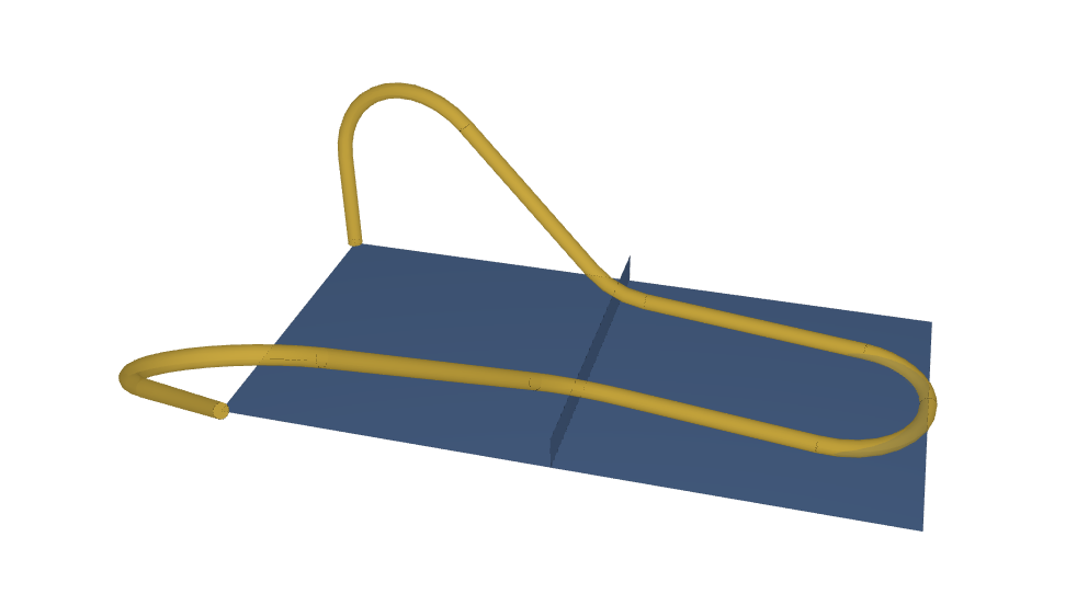
This class will be used to find the optimum thanks to optimizer.
2.3 - Create elementary generator & optimizer
To build our optimizer, we need to import some packages :
from random import random
import cma
In Optimize class, we would like to explain to you the aim of the Optimize method. At each line, there is a comment if needed.
- Concerning
cma.fmin, this function will find the best solution using 'self.objective' and an initialized vector solution. The method uses a vector that refers to position of point in order to respect condition concerning minimal radius.
    def optimize(self, assemblies: List[Assembly], number_solution_per_assembly:int)->List[Assembly]:
        solutions = []
        for assembly in assemblies: #we would find every best solutions concerning a list of assembly
            self.assembly = assembly

            x0a = [random() for i in range(len(self.assembly.frames))] #First vector to initialize solving

            check =True
            compt = 0
            number_solution = 0
            while check:
                xra, fx = cma.fmin(self.objective, x0a, 0.1,
                                   options={'bounds': [0, 1], #each point can be placed thanks to a percentage and the direction of each frame
                                            'tolfun': 1e-8, #precision of each solution returned by self.objective
                                            'verbose': 10,
                                            'ftarget': 1e-8, #if self.objective return is smaller than 'ftarget', a solution is found
                                            'maxiter': 10})[0:2] #maximum iteration wanted per searching, it chooses the best solution
                waypoints = self.assembly.waypoints
                radius = self.assembly.piping.genere_neutral_fiber(waypoints).radius #all radius characterizing neutral fiber
                min_radius = min(list(radius.values())) #we accept the solution with a 10% tolerance
                if min_radius >= 0.9*self.assembly.piping.minimum_radius and len(list(radius.keys())) == len(waypoints) - 2:
                    new_assembly = self.assembly.copy()
                    new_assembly.update(xra)
                    solutions.append(new_assembly)
                compt += 1
                number_solution += 1
                if compt == 20 or number_solution_per_assembly == number_solution:
                    break

        return solutions

    def objective(self, x):
        objective = 0
        self.update(x) #update assembly by a potential solution

        waypoints = self.assembly.waypoints
        radius = self.assembly.piping.genere_neutral_fiber(waypoints).radius
        min_radius = min(list(radius.values()))
        if min_radius < self.assembly.piping.minimum_radius:
            objective += 10 + (min_radius - self.assembly.piping.minimum_radius)**2 #penalization if a radius is smaller that expected
        else:
            objective += 10 - 0.1*(min_radius - self.assembly.piping.minimum_radius)

        return objective

    def update(self, x):
        self.assembly.update(x)
If you have more question concerning this part, we recommend you to read Simple power-transmission optimization.
2.4 - Build your workflow
First of all, in a workflow.py file, you have to create all assemblies you want to optimize. Each assembly will have something different, for example minimum radius allowed. Do not forget to import packages recommended :
import tutorials.tutorial5_piping as tuto
import volmdlr as vm
from dessia_common.workflow.core import Pipe, Workflow
from dessia_common.workflow.blocks import MethodType, InstantiateModel, MultiPlot, ModelMethod
Once done, we will begin the conscrution of workflow.
- Transform Optimizer object into workflow blocks.
block_optimizer = InstantiateModel(tuto.Optimizer, name='Optimizer')
block_optimize = ModelMethod(method_type=MethodType(tuto.Optimizer, 'optimize'), name='Optimize')
- In our case, elements are already generated and given to the optimizer. Now, we want to display in the platform some elements. Once elements generated in platform, we could see them thanks to a ParallelPlot.
list_attribute1 = ['length', 'min_radius', 'max_radius', 'distance_input', 'straight_line']
display_reductor = MultiPlot(selector_name="Multiplot", attributes=list_attribute1, name='Display')- We have all what we need, let's create the workflow.
#task order in workflow
block_workflow = [block_optimizer, block_optimize, display_reductor]
#connection in workflow
pipe_worflow = [Pipe(block_optimizer.outputs[0], block_optimize.inputs[0]),
Pipe(block_optimize.outputs[0], display_reductor.inputs[0])]
#last element refers to solutions
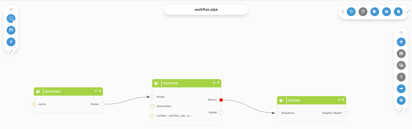
orkflow = Workflow(block_workflow, pipe_worflow, block_optimize.outputs[0], name="workflow pipe")
After creating your workflow, you can execute it by the following steps
f1 = vm.Frame3D(vm.Point3D(0.05, 0.1, 0), vm.Vector3D(1, 0, 0), vm.Vector3D(0, 1, 0), vm.Vector3D(0, 0, 1))
p1 = vm.surfaces.Plane3D(f1)
s1 = vm.surfaces.Surface2D(outer_contour=vm.wires.ClosedPolygon2D([vm.Point2D(-0.05, -0.1),
                                                                vm.Point2D(0.05, -0.1),
                                                                vm.Point2D(0.05, 0.1),
                                                                vm.Point2D(-0.05, 0.1)]),
                        inner_contours=[])
face1 = vm.shells.OpenShell3D([vm.faces.PlaneFace3D(surface3d=p1, surface2d=s1)])
face1.color = (92 / 255, 124 / 255, 172 / 255)
face1.alpha = 1

f2 = vm.Frame3D(vm.Point3D(0.05, 0.1, 0.005), vm.Vector3D(1, 0, 0), vm.Vector3D(0, 0, 1), vm.Vector3D(0, 1, 0))
p2 = vm.surfaces.Plane3D(f2)
s2 = vm.surfaces.Surface2D(outer_contour=vm.wires.ClosedPolygon2D([vm.Point2D(-0.05, -0.005),
                                                                vm.Point2D(0.05, -0.005),
                                                                vm.Point2D(0.05, 0.005),
                                                                vm.Point2D(-0.05, 0.005)]),
                        inner_contours=[])
face2 = vm.shells.OpenShell3D([vm.faces.PlaneFace3D(surface3d=p2, surface2d=s2)])
face2.color = (92 / 255, 124 / 255, 172 / 255)
face2.alpha = 1

vol = vm.core.VolumeModel([face1, face2])

housing = tuto.Housing(faces=[face1, face2], origin=vm.Point3D(0, 0, 0))

p1 = vm.Point3D(0, 0.1, 0.01)
p2 = vm.Point3D(0.05, 0.1, 0.01)
frame1 = tuto.Frame(start=p1, end=p2)

p1 = vm.Point3D(0.05, 0.1, 0.01)
p2 = vm.Point3D(0.1, 0.1, 0.01)
frame2 = tuto.Frame(start=p1, end=p2)

p1 = vm.Point3D(0, 0.2, 0)
p2 = vm.Point3D(0.05, 0.2, 0)
frame3 = tuto.Frame(start=p1, end=p2)

p1 = vm.Point3D(0.05, 0.2, 0)
p2 = vm.Point3D(0.1, 0.2, 0)
frame4 = tuto.Frame(start=p1, end=p2)

p1 = vm.Point3D(0, 0, 0)
p2 = vm.Point3D(0.1, 0, 0)
piping1 = tuto.Piping(start=p1, end=p2,
                      direction_start=vm.Vector3D(0, 0, 1), direction_end=vm.Vector3D(1, 0, 1),
                      diameter=0.005, length_connector=0.1, minimum_radius=0.03)
piping2 = tuto.Piping(start=p1, end=p2,
                      direction_start=vm.Vector3D(0, 0, 1), direction_end=vm.Vector3D(1, 0, 1),
                      diameter=0.005, length_connector=0.1, minimum_radius=0.05)

assemblies = []
minimum_radius = 0.02
for i in range(30):
    minimum_radius += 0.003
    p1 = vm.Point3D(0, 0, 0)
    p2 = vm.Point3D(0.1, 0, 0)
    for j in range(2):
        p1 += vm.Point3D(0.01, 0, 0)
        piping1 = tuto.Piping(start=p1, end=p2,
                              direction_start=vm.Vector3D(0, 0, 1), direction_end=vm.Vector3D(1, 0, 1),
                              diameter=0.005, length_connector=0.1, minimum_radius=0.03)
        assemblies.append(tuto.Assembly(frames=[frame1, frame3, frame4, frame2], piping=piping1, housing=housing))


# Workflow input
input_values = {workflow.index(block_optimize.inputs[1]): assemblies,
                workflow.index(block_optimize.inputs[2]): 1,
                }

 # run workflow
 workflow_run = workflow.run(input_values)
Workflow in your platform
To put your workflow in your platform, you have to type the following command after your workflow :
from dessia_api_client import Client
c = Client(api_url='<https://api.YOURPLATFORM.dessia.tech>')
r = c.create_object_from_python_object(workflow)
workflow is an instance of Workflow object.
Create your Workflow in platform
If you have not created your workflow locally (script) you can directly create it on the platform using the workflow builder, this way of doing things is the most recommended because it allows you to visualize the workflow being created and thus avoid making mistakes (for example in connecting ports), to do this you just need to install the application (package) on the platform (in this case tutorials) and requirements (see setup.py file in tutorials package) so that you have access to the class and methods and thus create your blocks. Note that you can export your workflow from the platform in script format if necessary.
Your workflow in platform: